itea.inspection

Interaction Transformation expression’s Inspector

Sub-module containing three classes to help inspect and explain the results obtained with the itea.

ITExpr_explainer: Implementations of feature importances methods specific to the Interaction-Transformation representation, and several visualization tools to help interpret the final expression;
ITExpr_inspector: Based on a more statistical approach, this class implements methods to measure the quality of the final expression by calculating information between individual terms;
ITExpr_texifier: Creation of latex representations of the final expression and its derivatives. In cases where the final expression is simple enough, the analysis of the expression can provide useful insights.

All the modules are designed to work with ITExpr`s. After the evolutionary process is performed (by calling `fit() on the ITEA_classifier or ITEA_regressor), the best final expression can be accessed by itea.bestsol_, and those classes are specialized in different ways of inspecting the final model.

Additionally, there is one class designed to work with the ´`itea``, instead of ITExpr expressions. The class ITEA_summarizer implements a method to automatically create a pdf file containing information generated with all the inspection classes, in an attempt to automate the task of generating an interpretability report.

Sub-module contents:

ITExpr_explainer
ITExpr_inspector
ITExpr_texifier
ITEA_summarizer

ITExpr_explainer 

class itea.inspection.ITExpr_explainer(*, itexpr, tfuncs, tfuncs_dx=None)[source]

Bases: object

Class to explain ITExpr expressions.

Constructor method.

Parameters

itexpr (ITExpr_regressor or ITExpr_classifier) – fitted instance of an ITExpr class to be explained.
tfuncs (dict) – transformations functions. Should always be a dict where the keys are the names of the transformation functions and the values are unary vectorized functions.
tfuncs_dx (dict, default=None) – derivatives of the given transformations functions, the same scheme. When set to None, the itea package will use automatic differentiation through jax to create the derivatives.

average_partial_effects(X)[source]

Feature importance estimation through the Partial Effects method.

This method attributes the importance to the i-th variable by using the mean value of the partial derivative w.r.t. i, evaluated for all data in X.

This method assumes that every feature is continuous.

The partial effect of a given variable for a function $f$ is calculated by:

$PE_j = \frac{\partial \widehat{f}}{\partial x_j} (\mathbf{x}, \mathbf{\beta}).$

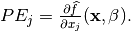
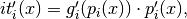
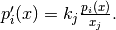
The IT expression can be automatically differentiated:

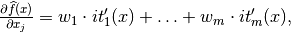
$\frac{\partial \widehat{f}(x)}{\partial x_j} = w_1 \cdot it'_1(x) + \ldots + w_m \cdot it'_m(x),$

where

$it'_i(x) = g'_i(p_i(x)) \cdot p'_i(x),$

$p'_i(x) = k_j\frac{p_i(x)}{x_j}.$

Parameters: X (numpy.array of shape (n_samples, n_features)) – data from which we want to extract the feature importance for the predicted outcomes of the model. If X is a single observation, the partial effects are calculated and returned directly. If X contains multiple observations, then the mean partial effect for each variable through all observations is returned.
Returns: ape_values – the importance of each feature of X, for each class found in the given itexpr. If itexpr is an ITExpr_regressor, then the returned array will have the shape (1, n_features).
Return type: numpy.array of shape (n_classes, n_features)

Notes

This feature importance measure is based on the paper: “Aldeia, G. & França, F. (2021). Measuring Feature Importance of Symbolic Regression Models GECCO.”

fit(X, y)[source]

Fit method to store the data used in the training of the given itexpr instance.

Parameters

X (array-like of shape (n_samples, n_features)) – data used to train the itexpr model.
y (array-like of shape (n_samples, )) – target data used to train the itexpr model.

Returns

self – explainer with a calculated covariance matrix, ready to generate plots and explanations.

Return type

ITExpr_explainer

Raises

NotFittedError – If the given itexpr is not fitted.
KeyError – If not all keys of tfuncs are contained in the keys of tfuncs_dx.

integrated_gradients(X, m_steps=300)[source]

Feature importance estimation through the Integrated Gradients method.

The idea of the integrated gradient is to calculate a local importance score for a feature $i$ by evaluating — given a baseline $\mathbf{x}'$ and a specific point $\mathbf{x}$ — the integral of the models’ gradients $\frac{\partial f}{\partial x_i}$ along a straight line between the baseline and the specific point. Since gradients describe how minimal local changes interfere with the model’s predictions, the calculated importance represents the accumulation of the gradient of each variable to go from the baseline to the specific point.

$IntegratedGrads_{i}^{approx} (\mathbf{x}) = \frac{(x_i - x_{i}')}{m} \sum_{k = 1}^{m} \frac{\partial \widehat {f} (\mathbf{x}' + \frac{k}{m}(\mathbf{x} - \mathbf{x}'))} {\partial x_i}$

In our implementation, the baseline used is the average value of the training attributes used in fit(X_train, y_train), thus the calculated value is close to SHAP.

Parameters

X (numpy.array of shape (n_samples, n_features)) – data from which we want to extract the feature importance for the predicted outcomes of the model. If X is a single observation, the integrated gradients are calculated and returned directly. If X contains multiple observations, then the mean integrated gradients for each variable through all observations is returned.
m_steps (int, default=300) – number of steps $m$ used in the Riemman summation approximation of the integral. Small values leads to a poor approximation, while higher values decreases the error at the cost of a higher computational cost.

Returns

ig – the importance of each feature of X, for each class found in the given itexpr. If itexpr is an ITExpr_regressor, then the returned array will have the shape (1, n_features).

Return type

numpy.array of shape (n_classes, n_features)

Notes

The Integrated Gradient method was proposed in the paper: “Mukund Sundararajan, Ankur Taly, and Qiqi Yan. 2017. Axiomatic attribution for deep networks. In Proceedings of the 34th International Conference on Machine Learning - Volume 70 (ICML’17). JMLR.org, 3319–3328.”

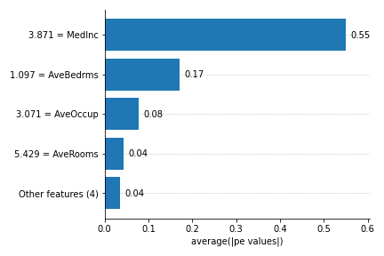
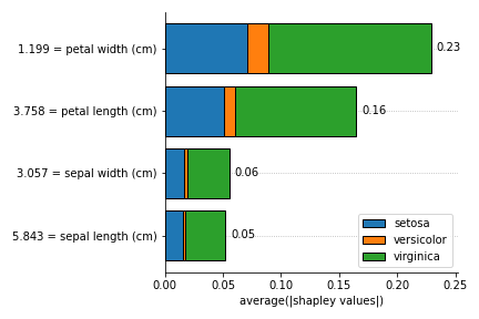
plot_feature_importances(X, *, barh_kw=None, ax=None, grouping_threshold=0.05, target=None, importance_method='pe', show_avg_values=True, show=True)[source]

Bar plot of the feature importance, that can be calculated with the Partial effects (PE) or Shapley Values (shapley).

Parameters

X (array-like of shape (n_samples, n_features)) – data to explain.
bar_kw (dict or None, default=None) – dictionary with keywords to be used when generating the plots. When set to None, then bar_kw= {'alpha':1.0, 'align':'center'}.
ax (matplotlib.axes or None, default=None) – axis to generate the plot. If none is given, then a new axis is created. if is a single axis, the plot will be drawn within the given axis. The new axis and figure created can be accessed through the axes_ and figure_ attributes. Notice that, if multiple plot functions were called, then axes_ and figure_ corresponds to the latest plot generated.
grouping_threshold (float, default = 0.05) – The features will be iterated in order of importance, from the smallest to the highest importance, and a group of the smallest features that sum up less than the given percentage of importance will be grouped to reduce the plot information. To disable the creation of the group, set grouping_threshold=0.
target (string, int, list[strings], list[ints] or None, default=None) – The targets to be considered when generating the plot for ITExpr_classifier. If the training data used strings as targets on y, then the target must be a string of a valid class or a list of valid classes. If the training data was encoded as integers, then the target must be an int or a list of integers. This argument is ignored if the itexpr is an ITExpr_regressor.
importance_method (string, default='pe') – string specifying which method should be used to estimate feature importance. Available methods are: ['pe', 'shapley', 'ig'].
show_avg_values (bool, default=True) – determines if the average feature value should be displayed left to the feature names in the y axis.
show (bool, default=True) – boolean value indicating if the generated plot should be displayed or not.

Raises

ValueError – If ax or target has invalid values.

Notes

This plot is heavily inspired by the bar plot from the SHAP package

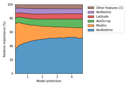
plot_normalized_partial_effects(*, num_points=20, grouping_threshold=0.05, stack_kw=None, ax=None, show=True)[source]

Partial effects plots, separing the training data into discrete intervals.

First, the output interval is discretized. Then, for each interval, the partial effect of the sample data that predict values within the interval is calculated. Finally, they are normalized in order to make the total contribution by 100%.

_images/plot_normalized_partial_effects_1.png

Parameters

num_points (int, default = 20) – the number of points to divide the interval when generating the plots. The value must be equal or greater than 2. Large values can end up creating intervals where no predictions in the training data lies within resulting in points that are not evenly distributed, or in a noisy plot. The adequate number of points can be different for each dataset. This parameter is ignored if itexpr == ITExpr_classifier.
grouping_threshold (float, default = 0.05) – The features will be iterated in order of importance, from the smallest to the highest importance, and a group of the smallest features that sum up less than the given percentage of importance will be grouped to reduce the plot information. To disable the creation of the group, set grouping_threshold=0.
stack_kw (dict or None, default=None) – dictionary with keywords to be used when generating the plots. When set to None, then stack_kw is {'baseline': 'zero', 'labels': labels, 'edgecolor': 'k', 'alpha': 0.75}.
ax (matplotlib.axes or None, default=None) – axis to generate the plot. If none is given, then a new axis is created. if is a single axis, the plot will be drawn within the given axis. The new axis and figure created can be accessed through the axes_ and figure_ attributes. Notice that, if multiple plot functions were called, then axes_ and figure_ corresponds to the latest plot generated.
show (bool, default=True) – boolean value indicating if the generated plot should be displayed or not.

Raises

ValueError – If ax has invalid values.

Notes

This plot was inspired by the relative feature contribution plot reported in the paper: “R. M. Filho, A. Lacerda and G. L. Pappa, “Explaining Symbolic Regression Predictions,” 2020 IEEE Congress on Evolutionary Computation (CEC)”.

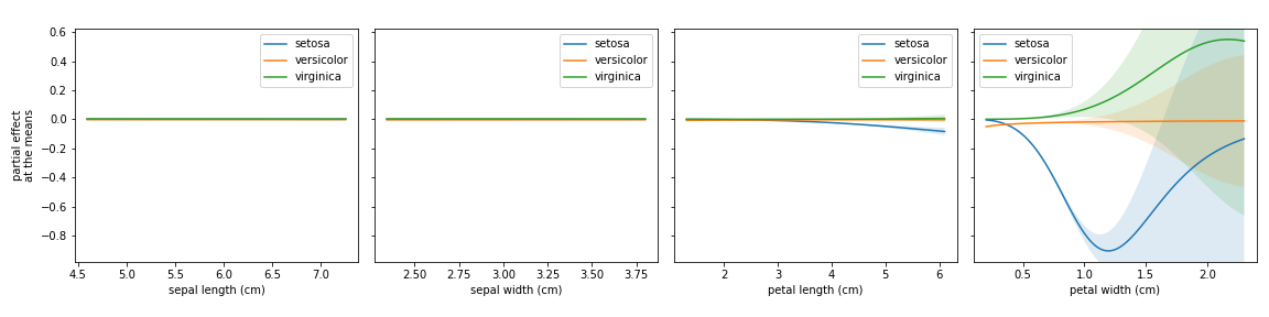
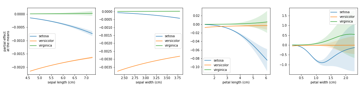
plot_partial_effects_at_means(*, X, features, percentiles=(5, 95), num_points=100, n_cols=3, target=None, line_kw=None, fill_kw=None, ax=None, show_err=True, share_y=True, rug=True, show=True)[source]

Partial effects plots for the given features, when their co-variables are fixed at the mean.

_images/plot_partial_effects_at_means_1.png

_images/plot_partial_effects_at_means_2.png

Parameters

X (numpy.array of shape (n_samples, n_features)) – data from which we want to extract the feature importance for the predicted outcomes of the model.
features (string, list[string], int, list[int] or None, default=None) – the features to generate the plots. It can be a single feature referred to by its label or its index or a list of features.
percentiles (tuple of ints, default=(5, 95)) – the quartiles interval to generate the plot.
num_points (int, default = 100) – the number of points to divide the interval when generating the plots.
n_cols (int, default=3) – number of columns to be used when creating the plot grids if ax is None.
target (string, int, list[strings], list[ints] or None, default=None) – The targets to be considered when generating the plot for ITExpr_classifier. If the training data used strings as targets on y, then the target must be a string of a valid class or a list of valid classes. If the training data was encoded as integers, then the target must be an int or a list of integers. This argument is ignored if the itexpr is an ITExpr_regressor.
line_kw (dict or None, default=None) – dictionary with keywords to be used when generating the plots. When set to None, then line_kw= {}.
fill_kw (dict or None, default=None) – dictionary with keywords to be used when generating the plots. When set to None, then fill_kw= {'alpha' : 0.15}.
ax (matplotlib.axes or list of matplotlib.axes or None, default=None) – axis to generate the plot. If none is given, then a new axis is created. If is a single axis, the plot will be drawn within the given axis. If ax is a list, then it must have the same number of elements in features. The new axis and figure created can be accessed through the axes_ and figure_ attributes. Notice that, if multiple plot functions were called, then axes_ and figure_ corresponds to the latest plot generated.
show_err (bool, default=True) – boolean variable indicating if the standard error should be plotted.
share_y (bool, default True) – boolean variable to specify if the axis should have the same interval on the y axis.
rug (bool, default True) – whether to show the distribution as a rug. The input data will be divided into 10 deciles, which will be showed right above the x axis line.
show (bool, default=True) – boolean value indicating if the generated plot should be displayed or not.

Raises

ValueError – If ax or target has invalid values.
IndexError – If one or more specified features are not in explainer.itexpr labels.

Notes

This plot is heavily inspired by the Partial Dependency Plot from scikit-learn.

selected_features(idx=False)[source]

Method to identify if any of the original features were left out of the IT expression during the evolution of the exponents’ array.

Parameters: idx (bool, default=False) – boolean variable specifying if the method should return a list with the labels of the features or their indexes.
Returns: selected – array containing the labels of the features that are present in the model, or their indexes if idx=True.
Return type: array of shape (n_selected_features)

shapley_values(X)[source]

Feature importance estimation through approximation of the Shapley values with the gradient information.

The shapley values come from the coalitional game theory and were proposed as a feature importance measures by Scott Lundberg in “Scott M. Lundberg and Su-In Lee. 2017. A unified approach to interpreting model predictions. NIPS”. The equation:

$\phi_j(x) = \sum_{Q \subseteq S \setminus \left\{j\right\}} {\frac{|Q|!(|S| - |Q| - 1)!}{|S|!} (\Delta_{Q \cup \{j\}}(x) - \Delta_{Q}(x))},$

where $S$ is the set of variables, $\Delta_Q$ is the contribution of the set $Q$ , the difference between the prediction when we fix the values of $Q$ , and the expected prediction.

It is possible to approximate these values by the equation:

$\widehat{\phi_j}(x) = \mathbb{E}[PE_j] \cdot (x_j - \mathbb{E}[x_j]),$

Where $PE_j$ is the partial effect w.r.t $j$ .

Parameters: X (numpy.array of shape (n_samples, n_features)) – data from which we want to extract the feature importance for the predicted outcomes of the model. If X is a single observation, the shapley values are calculated and returned directly. If X contains multiple observations, then the mean shapley value for each variable through all observations is returned.
Returns: shapley_values – the importance of each feature of X, for each class found in the given itexpr. If itexpr is an ITExpr_regressor, then the returned array will have the shape (1, n_features).
Return type: numpy.array of shape (n_classes, n_features)

Notes

The shapley values are described and explained in: “Scott M. Lundberg and Su-In Lee. 2017. A unified approach to interpreting model predictions. NIPS”

The approximation of shapley values by means of the partial effect was studied in the paper: This feature importance measure is based on the paper: “Aldeia, G. & França, F. (2021). Measuring Feature Importance of Symbolic Regression Models GECCO.”

ITExpr_inspector 

class itea.inspection.ITExpr_inspector(*, itexpr, tfuncs, decimal_places=3)[source]

Bases: object

class ITExpr_inspector.

Based on a more statistical approach, this class implements methods to measure the quality of the final expression by calculating information between individual terms.

Constructor method.

Parameters

itexpr (ITExpr_regressor or ITExpr_classifier) – fitted instance of an ITExpr class to be explained.
tfuncs (dict) – transformations functions. Should always be a dict where the keys are the names of the transformation functions and the values are unary vectorized functions.

fit(X, y)[source]

Fit method to store the data used in the training of the given itexpr instance.

Parameters

X (array-like of shape (n_samples, n_features)) – data used to train the itexpr model.
y (array-like of shape (n_samples, )) – target data used to train the itexpr model.

Returns

self – inspector with the calculated covariance matrix.

Return type

ITExpr_inspector

terms_analysis()[source]

Method to calculate different metrics for the terms composing the IT expression.

Returns

analysis – returns a dictionary containing several term information and metrics calculated for each term:

coef: coefficient of each term (or coefficients, if the itexpr is an instance of ITExpr_classifier);
func: transformation function of each term;
strengths: the exponents of each term;
coef stderr.: the standard error of the coefficients;
mean pairwise disentanglement: the mean disentanglement between each term when compared with the others;
mean mutual information: the mean continuous mutual information between each term when compared with the others;
prediction var.: the variance of the predicted outcomes for each term when predicting the training data.

Return type

dict

ITExpr_texifier 

class itea.inspection.ITExpr_texifier[source]

Bases: object

class containing static methods to create LaTeX representations of the expression.

static derivatives_to_latex(itexpr, term_separator=' + ', term_wrapper=None)[source]

Static method that takes an instance of an ITExpr and returns a list containing a latex representation of each partial derivative of the expression.

Parameters

itexpr (ITExpr_classifier or ITExpr_regressor) – an instance of itexpr to be texified.
term_separator (string, default=' + ') – string to be used to concatenate each term.
term_wrapper (None or Callable, default=None) –
a function that takes two arguments: i the index of the term and term the term itself, and returns a string. This can be used to add special formatations to the terms. Examples are:
- lambda i, term: r'\underbrace{'+term+r'} _{\text{term '+str(i)+'}}' to add a underbracket with the index of the term;
- lambda i, term: term to do nothing;
When set to None, then the latter expression will be used.

Returns

itexpr_latexs – list of strings, where each string is a latex representation of the partial derivative of the given itexpr.

Return type

list[string]

static to_latex(itexpr, term_separator=' + ', term_wrapper=None)[source]

Static method that takes an instance of an ITExpr and returns a latex representation of the expression.

Parameters

itexpr (ITExpr_classifier or ITExpr_regressor) – an instance of itexpr to be texified.
term_separator (string, default=' + ') – string to be used to concatenate each term.
term_wrapper (None or Callable, default=None) –
a function that takes two arguments: i the index of the term and term the term itself, and returns a string. This can be used to add special formatting to the terms. Examples are:
- lambda i, term: r'\underbrace{'+term+r'} _{\text{term '+str(i)+'}}' to add a underbracket with the index of the term;
- lambda i, term: term to do nothing;
When set to None, then the latter expression will be used.

Returns

itexpr_latex – latex expression representing the given itexpr.

Return type

string

ITEA_summarizer 

class itea.inspection.ITEA_summarizer(*, itea)[source]

Bases: object

Class to automatically generate a pdf file reporting several interpretability plots for the expression.

Constructor method.

Parameters: itea (ITEA_classifier or ITEA_regressor) – fitted instance of an ITEA class to be summarized.

autoreport(importance_methods=None, save_path='.', name_suffix='', use_temp_folder=True)[source]

automatically generate a pdf using the methods implemented in ITExpr_inspector, ITExpr_explainer, and ITExpr_texifier.

The idea is to simplify the generation of the plots and tables, removing from the user the need to understand, instantiate the classes and call the plots functions.

All explanations are generated with the training data, and every item in the report can be obtained manually by using the ITExpr_inspector, ITExpr_explainer, and ITExpr_texifier.

This method makes usage of the PyLaTeX package and requires a visible latex installation to work properly.

The .tex file used to generate the pdf will also be saved on the designed path.

You can download one example of report by clicking here.

Parameters

importance_methods (string or list[strings] or None, default=None) – Feature importance method(s) used to generate explanations in the report. Must be one of the possible explainers implemented (['pe', 'ig', 'shapley']) or a list containing one or more of the explainers. If None, then 'pe' will be used. The report will contain one page for each method specified here.
save_path (string, default='.') – path to save the pdf report. The file will be saved as “Report.pdf”, unless a name_suffix is provided. A Te
name_suffix (string, default="") – suffix to add in the name of the report.
use_temp_folder (boolean, defaut=True) – specifies if a temporary folder should be used to save the plots during the creation of the report. If false, then the plots will be saved on the save_path.

fit(X, y)[source]

Fit method to store the data used in the training of the given itea instance.

Parameters

X (array-like of shape (n_samples, n_features)) – data used to train the itexpr model.
y (array-like of shape (n_samples, )) – target data used to train the itexpr model.

Returns

self

Return type

ITEA_summarizer

plot_convergence(*, data=None, n_cols=1, line_kw=None, fill_kw=None, ax=None, show_err=True, show=True)[source]

Plot of information about the itea evolutionary process. This function is intended to help visualize the information on the itea.convergence_ dictionary.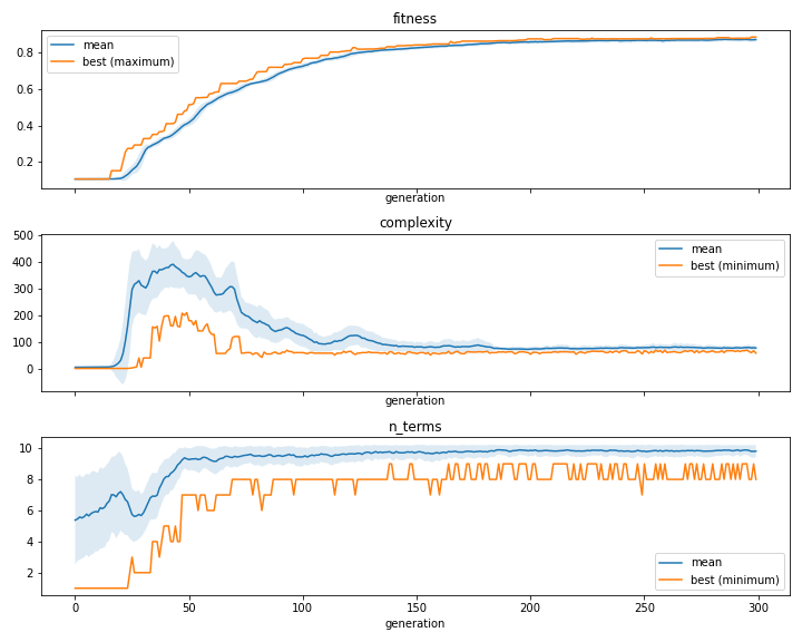

Parameters

data (string, list of string, or None, default=None) – the convergence information to generate the plots. It can be a single string or a list with strings in ['fitness', 'n_terms', 'complexity']. If set to none, then the whole list of strings will be used.
n_cols (int, default=1) – number of columns to be used when creating the plot grids if ax is None.
line_kw (dict or None, default=None) – dictionary with keywords to be used when generating the plots. When set to None, then line_kw= {}.
fill_kw (dict or None, default=None) – dictionary with keywords to be used when generating the plots. When set to None, then fill_kw= {'alpha' : 0.15}.
ax (matplotlib.axes or list of matplotlib.axes or None, default=None) – axis to generate the plot. If none is given, then a new axis is created. If is a single axis, the plot will be drawn within the given axis. If ax is a list, then it must have the same number of elements in data.
show_err (bool, default=True) – boolean variable indicating if the standard error should be plotted.
show (bool, default=True) – boolean value indicating if the generated plot should be displayed or not.

Raises

ValueError – If ax or data has invalid values.

itea.inspection

ITExpr_explainer

ITExpr_inspector

ITExpr_texifier

ITEA_summarizer

ITExpr_explainer 

ITExpr_inspector 

ITExpr_texifier 

ITEA_summarizer 