Interacting with ProtoDash
In this notebook we’ll combine the ProtoDash and the Partial Effects to obtain feature importances on the digits classifications task.
ProtoDash was proposed in Gurumoorthy, Karthik & Dhurandhar, Amit & Cecchi, Guillermo & Aggarwal, Charu. (2019). Efficient Data Representation by Selecting Prototypes with Importance Weights. 260-269. 10.1109/ICDM.2019.00036.
[1]:
import numpy  as np
import pandas as pd

# automatically differentiable implementation of numpy
import jax.numpy as jnp # v0.2.13

import shap #0.34.0

from sklearn.metrics import classification_report
from sklearn         import datasets

from sklearn.model_selection import train_test_split
from IPython.display         import display

import matplotlib.pyplot as plt

from itea.classification import ITEA_classifier
from itea.inspection     import *

from sklearn.preprocessing import OneHotEncoder

from aix360.algorithms.protodash import ProtodashExplainer #0.2.1

import warnings
warnings.filterwarnings(action='ignore', module=r'itea')
[2]:
digits_data = datasets.load_digits(n_class=10)

X, y        = digits_data['data'], digits_data['target']
labels      = digits_data['feature_names']
targets     = digits_data['target_names']

X /= X.max(axis=1).reshape(-1, 1)

X_train, X_test, y_train, y_test = train_test_split(
    X, y, test_size=0.33, random_state=42)

tfuncs = {
    'id' : lambda x: x,
    'sin': jnp.sin,
    'cos': jnp.cos,
    'tan': jnp.tan
}

clf = ITEA_classifier(
    gens            = 100,
    popsize         = 100,
    max_terms       = 40,
    expolim         = (0, 2),
    verbose         = 10,
    tfuncs          = tfuncs,
    labels          = labels,
    simplify_method = None,
    random_state    = 42,
    fit_kw          = {'max_iter' : 5}
).fit(X_train, y_train)

final_itexpr = clf.bestsol_
final_itexpr.selected_features_
gen | smallest fitness | mean fitness | highest fitness | remaining time
----------------------------------------------------------------------------
  0 |         0.105569 |     0.105569 |        0.105569 | 9min40sec
 10 |         0.105569 |     0.105569 |        0.105569 | 9min8sec
 20 |         0.105569 |     0.105669 |        0.107232 | 7min4sec
 30 |         0.107232 |     0.111380 |        0.133001 | 6min41sec
 40 |         0.133001 |     0.146708 |        0.152120 | 6min11sec
 50 |         0.152120 |     0.154530 |        0.227764 | 6min19sec
 60 |         0.227764 |     0.227839 |        0.230258 | 5min34sec
 70 |         0.324190 |     0.335553 |        0.351621 | 4min23sec
 80 |         0.351621 |     0.396259 |        0.428928 | 5min27sec
 90 |         0.444722 |     0.467548 |        0.517872 | 2min53sec
[2]:
array(['pixel_0_0', 'pixel_0_1', 'pixel_0_2', 'pixel_0_3', 'pixel_0_4',
       'pixel_0_5', 'pixel_0_6', 'pixel_0_7', 'pixel_1_0', 'pixel_1_1',
       'pixel_1_2', 'pixel_1_3', 'pixel_1_4', 'pixel_1_5', 'pixel_1_6',
       'pixel_1_7', 'pixel_2_0', 'pixel_2_1', 'pixel_2_2', 'pixel_2_3',
       'pixel_2_4', 'pixel_2_5', 'pixel_2_6', 'pixel_2_7', 'pixel_3_0',
       'pixel_3_1', 'pixel_3_2', 'pixel_3_3', 'pixel_3_4', 'pixel_3_5',
       'pixel_3_6', 'pixel_3_7', 'pixel_4_0', 'pixel_4_1', 'pixel_4_2',
       'pixel_4_3', 'pixel_4_4', 'pixel_4_5', 'pixel_4_6', 'pixel_4_7',
       'pixel_5_0', 'pixel_5_1', 'pixel_5_2', 'pixel_5_3', 'pixel_5_4',
       'pixel_5_5', 'pixel_5_6', 'pixel_5_7', 'pixel_6_0', 'pixel_6_1',
       'pixel_6_2', 'pixel_6_3', 'pixel_6_4', 'pixel_6_5', 'pixel_6_6',
       'pixel_6_7', 'pixel_7_0', 'pixel_7_1', 'pixel_7_2', 'pixel_7_3',
       'pixel_7_4', 'pixel_7_5', 'pixel_7_6', 'pixel_7_7'], dtype='<U9')
[3]:
print(classification_report(
    y_test,
    final_itexpr.predict(X_test),
    target_names=[str(t) for t in targets]
))
              precision    recall  f1-score   support

           0       0.54      0.64      0.58        55
           1       0.70      0.80      0.75        55
           2       0.53      0.44      0.48        52
           3       0.29      0.71      0.41        56
           4       0.69      0.69      0.69        64
           5       0.61      0.52      0.56        73
           6       0.58      0.49      0.53        57
           7       0.43      0.53      0.48        62
           8       0.40      0.19      0.26        52
           9       0.27      0.04      0.08        68

    accuracy                           0.50       594
   macro avg       0.51      0.51      0.48       594
weighted avg       0.51      0.50      0.48       594
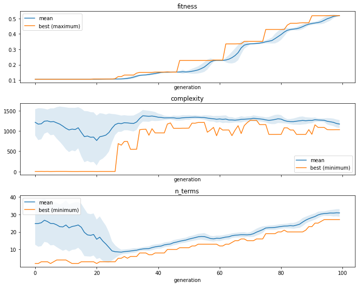
We can use the ITEA_summarizer to inspect the convergence during the evolution. In the cell below, we’ll create 3 plots, one for the fitness (classification accuracy), one for the complexity (number of nodes if the IT expression was converted to a symbolic tree) and number of terms (number of IT terms of the solutions in the population for each generation).
[4]:
fig, ax = plt.subplots(3, 1, figsize=(10, 8), sharex=True)

summarizer = ITEA_summarizer(itea=clf).fit(X_train, y_train).plot_convergence(
    data=['fitness', 'complexity', 'n_terms'],
    ax=ax,
    show=False
)

plt.tight_layout()
plt.show()
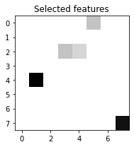
[5]:
# features are named pixel_x_y. Lets extract those coordinates and
# paint in a figure to show the selected features

selected_features = np.zeros((8, 8))
for feature_name, feature_importance in zip(
    final_itexpr.selected_features_,
    np.sum(final_itexpr.feature_importances_, axis=0)
):
    x, y = feature_name[-3], feature_name[-1]
    selected_features[int(x), int(y)] = feature_importance

fig, axs = plt.subplots(1, 1, figsize=(3,3))

axs.imshow(selected_features, cmap='gray_r')
axs.set_title(f"Selected features")

plt.tight_layout()
plt.show()
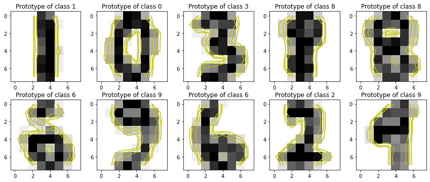
[6]:
onehot_encoder = OneHotEncoder(sparse=False)
onehot_encoded = onehot_encoder.fit_transform(
    np.hstack( (X_train, y_train.reshape(-1, 1)) ) )

explainer = ProtodashExplainer()

# call protodash explainer. We'll select 10 prototypes
# S contains indices of the selected prototypes
# W contains importance weights associated with the selected prototypes
(W, S, _) = explainer.explain(onehot_encoded, onehot_encoded, m=10)
elementwise comparison failed; returning scalar instead, but in the future will perform elementwise comparison
elementwise comparison failed; returning scalar instead, but in the future will perform elementwise comparison
elementwise comparison failed; returning scalar instead, but in the future will perform elementwise comparison
elementwise comparison failed; returning scalar instead, but in the future will perform elementwise comparison
[7]:
from matplotlib import cm

fig, axs = plt.subplots(2, 5, figsize=(12,5))

# Showing 10 prototypes
for s, ax in zip(S, fig.axes):
    ax.imshow(X_train[s].reshape(8, 8), cmap='gray_r')
    ax.set_title(f"Prototype of class {y_train[s]}")

    Z = X_train[s].reshape(8, 8)
    levels = [0.1, 0.2, 0.4]

    norm = cm.colors.Normalize(vmax=abs(Z).max(), vmin=-abs(Z).max())
    cmap = cm.PRGn

    cset2 = ax.contour(Z, levels, colors='y')

    for c in cset2.collections:
        c.set_linestyle('solid')


plt.tight_layout()
plt.show()
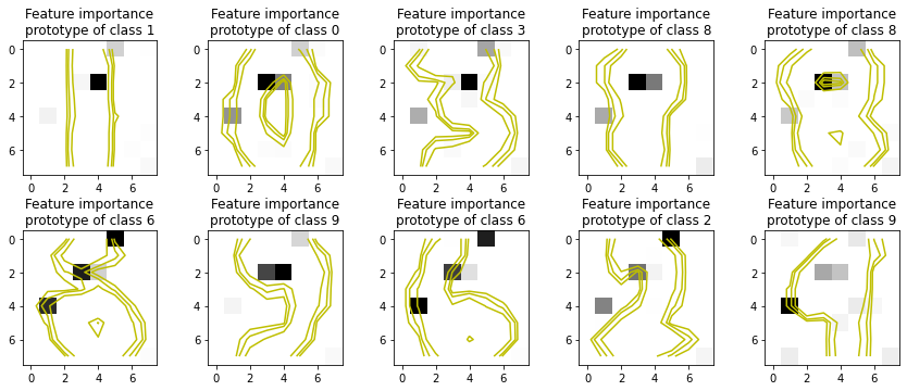
[8]:
it_explainer = ITExpr_explainer(
    itexpr=final_itexpr,
    tfuncs=tfuncs
).fit(X_train, y_train)

fig, axs = plt.subplots(2, 5, figsize=(12,5))

for s, ax in zip(S, fig.axes):

    importances = it_explainer.average_partial_effects(X_train[s, :].reshape(1, -1))[y_train[s]]

    ax.imshow(importances.reshape(8, 8), cmap='gray_r')
    ax.set_title(f"Feature importance\nprototype of class {y_train[s]}")

    Z = X_train[s].reshape(8, 8)
    levels = [0.1, 0.2, 0.4]

    norm = cm.colors.Normalize(vmax=abs(Z).max(), vmin=-abs(Z).max())
    cmap = cm.PRGn

    cset2 = ax.contour(Z, levels, colors='y')

    for c in cset2.collections:
        c.set_linestyle('solid')

plt.tight_layout()
plt.show()

[9]:
shap_explainer = shap.KernelExplainer(
    final_itexpr.predict,
    shap.sample(pd.DataFrame(X_train, columns=labels), 100)
)

fig, axs = plt.subplots(2, 5, figsize=(12,5))

for s, ax in zip(S, fig.axes):

    importances = np.abs(shap_explainer.shap_values(
            X_train[s, :].reshape(1, -1), silent=True, l1_reg='num_features(10)'))

    ax.imshow(importances.reshape(8, 8), cmap='gray_r')
    ax.set_title(f"Feature importance\nprototype of class {y_train[s]}")

    Z = X_train[s].reshape(8, 8)
    levels = [0.1, 0.2, 0.4]

    norm = cm.colors.Normalize(vmax=abs(Z).max(), vmin=-abs(Z).max())
    cmap = cm.PRGn

    cset2 = ax.contour(Z, levels, colors='y')

    for c in cset2.collections:
        c.set_linestyle('solid')

plt.tight_layout()
plt.show()
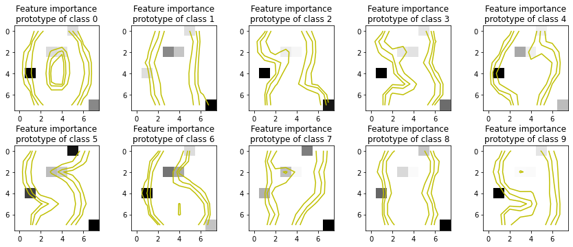
[10]:
it_explainer = ITExpr_explainer(
    itexpr=final_itexpr,
    tfuncs=tfuncs
).fit(X_train, y_train)

fig, axs = plt.subplots(2, 5, figsize=(12,5))

for c, ax in zip(final_itexpr.classes_, fig.axes):

    c_idx = np.array([i for i in range(len(y_train)) if y_train[i]==c])

    importances = it_explainer.average_partial_effects(X_train[c_idx, :])[c]

    ax.imshow(importances.reshape(8, 8), cmap='gray_r')
    ax.set_title(f"Feature importance\nprototype of class {c}")

    Z = X_train[c_idx, :].mean(axis=0).reshape(8, 8)
    levels = [0.1, 0.2, 0.4]

    norm = cm.colors.Normalize(vmax=abs(Z).max(), vmin=-abs(Z).max())
    cmap = cm.PRGn

    cset2 = ax.contour(Z, levels, colors='y')

    for c in cset2.collections:
        c.set_linestyle('solid')

plt.tight_layout()
plt.show()