Iris classification
This notebook will walk through the process of using the ITEA for classification (ITEA_classifier) and interpreting the final expression with the itea.inspection tools.
[1]:
import numpy  as np
import pandas as pd

# automatically differentiable implementation of numpy
import jax.numpy as jnp # v0.2.13

import matplotlib.pyplot as plt

from sklearn import datasets
from sklearn.metrics import classification_report

from sklearn.model_selection import train_test_split
from IPython.display         import display, Latex

from itea.classification import ITEA_classifier
from itea.inspection     import *

import warnings
warnings.filterwarnings(action='ignore', module=r'itea')
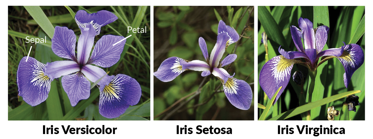
We will use the Iris data set in this example.
This data set contains 3 different classes of Iris flowers and has 4 features: sepal width, sepal length, petal width, and petal length.
One example of each flower is illustrated in the figure below.
Creating and fitting an ITEA_classifier
In this execution, we will fix the random_state argument to allow reproductible executions of the ITEA algorithm.
The IT expression is used as the decision function in a logistic regression. The inner logistic regression uses the saga solver described in “Defazio, A., Bach F. & Lacoste-Julien S. (2014). SAGA: A Fast Incremental Gradient Method With Support for Non-Strongly Convex Composite Objectives”.
The method will solve a multinomial classification problem with the softmax funcion applied over the decision function. By default, no regularization os performed (although the user can controlate this by setting values to alpha and beta parameters), and a maximum of 100 iterations of the saga solver is performed for each expression.
[2]:
iris_data = datasets.load_iris()
X, y      = iris_data['data'], iris_data['target']
labels    = iris_data['feature_names']
targets   = iris_data['target_names']

# changing numbers to the class names
y_targets = [targets[yi] for yi in y]

X_train, X_test, y_train, y_test = train_test_split(
    X, y_targets, test_size=0.33, random_state=42)

# Creating transformation functions for ITEA using jax.numpy
# (so we don't need to analytically calculate its derivatives)
tfuncs = {
    'id'       : lambda x: x,
    'sqrt.abs' : lambda x: jnp.sqrt(jnp.abs(x)),
    'log'      : jnp.log,
    'exp'      : jnp.exp
}

clf = ITEA_classifier(
    gens            = 50,
    popsize         = 50,
    max_terms       = 2,
    expolim         = (-1, 1),
    verbose         = 5,
    tfuncs          = tfuncs,
    labels          = labels,
    simplify_method = 'simplify_by_var',
    fit_kw          = {'max_iter':100},
    random_state    = 42,
).fit(X_train, y_train)
gen | smallest fitness | mean fitness | highest fitness | remaining time
----------------------------------------------------------------------------
  0 |         0.560000 |     0.848200 |        0.970000 | 0min32sec
  5 |         0.740000 |     0.961800 |        0.980000 | 0min22sec
 10 |         0.790000 |     0.969400 |        0.990000 | 0min23sec
 15 |         0.950000 |     0.982200 |        0.990000 | 0min17sec
 20 |         0.890000 |     0.982200 |        0.990000 | 0min18sec
 25 |         0.860000 |     0.982400 |        0.990000 | 0min18sec
 30 |         0.930000 |     0.981800 |        0.990000 | 0min11sec
 35 |         0.960000 |     0.982600 |        0.990000 | 0min8sec
 40 |         0.940000 |     0.981600 |        0.990000 | 0min5sec
 45 |         0.660000 |     0.973800 |        0.990000 | 0min2sec
Since the ITEA_classifier and the best solution found by the ITEA ITExpr_classifier are both scikit-like models, we can use some base methods like get_params.
In the cell below we inspect the parameters of the best expression. We can see the logistic regression regularization parameters (alpha and beta), the maximum number of iterations of the coefficients adjustment algorithm (max_iter), and the array of IT terms (expr), containing the terms that are being used to create the decision function for the logistic regression.
[3]:
# clf.get_params()          returns the ITEA parameters
# clf.bestsol_.get_params() returns the best expression parameters

clf.bestsol_.get_params()
[3]:
{'alpha': 0.0,
 'beta': 0.0,
 'expr': [('id', [0, -1, 1, 1]), ('id', [1, -1, -1, 0])],
 'fitness_f': None,
 'labels': array(['sepal length (cm)', 'sepal width (cm)', 'petal length (cm)',
        'petal width (cm)'], dtype='<U17'),
 'max_iter': 100,
 'tfuncs': {'id': <function __main__.<lambda>(x)>,
  'sqrt.abs': <function __main__.<lambda>(x)>,
  'log': <function jax._src.numpy.lax_numpy._one_to_one_unop.<locals>.<lambda>(x)>,
  'exp': <function jax._src.numpy.lax_numpy._one_to_one_unop.<locals>.<lambda>(x)>}}
Inspecting the results from ITEA_classifier and ITExpr_classifier
Now that we have fitted the ITEA, our clf contains the bestsol_ attribute, which is a fitted instance of ITExpr_classifier ready to be used.
[4]:
final_itexpr = clf.bestsol_

final_itexpr.to_str(term_separator='\n')
[4]:
'[-5.254 0.243 5.012]*id(sepal width (cm)^-1 * petal length (cm) * petal width (cm))\n[ 5.245 0.224 -5.469]*id(sepal length (cm) * sepal width (cm)^-1 * petal length (cm)^-1)\n[ 4.124 3.503 -7.627]'
[5]:
print(classification_report(
    y_test,
    final_itexpr.predict(X_test),
    target_names=targets
))
              precision    recall  f1-score   support

      setosa       1.00      1.00      1.00        19
  versicolor       0.94      1.00      0.97        15
   virginica       1.00      0.94      0.97        16

    accuracy                           0.98        50
   macro avg       0.98      0.98      0.98        50
weighted avg       0.98      0.98      0.98        50
We can use the ITExpr_inspector to obtain metrics regarding the IT terms in the expression
[6]:
display(pd.DataFrame(
    ITExpr_inspector(
        itexpr=final_itexpr, tfuncs=tfuncs
    ).fit(X_train, y_train).terms_analysis()
))
| coef | func | strengths | coef\nstderr. | mean pairwise\ndisentanglement | mean mutual\ninformation | prediction\nvar. | |
|---|---|---|---|---|---|---|---|
| 0 | [-5.254 0.243 5.012] | id | [0, -1, 1, 1] | [3.978 1.134 1.431] | 0.766 | 0.905 | [63.693 0.136 57.947] |
| 1 | [ 5.245 0.224 -5.469] | id | [1, -1, -1, 0] | [14.394 7.012 10.91 ] | 0.766 | 0.905 | [2.26 0.004 2.458] |
| 2 | [ 4.124 3.503 -7.627] | intercept | --- | [13.579 6.165 7.181] | 0.000 | 0.000 | [0. 0. 0.] |
By using the ITExpr_texifier, we can create formatted LaTeX strings of the final expression and its derivatives.
[7]:
# The final expression
display(Latex(
    '$ ITExpr = ' + ITExpr_texifier.to_latex(
        final_itexpr,
        term_wrapper=lambda i, term: r'\underbrace{' + term + r'}_{\text{term ' + str(i) + '}}'
    ) + '$'
))

[8]:
# List containing the partial derivatives
derivatives_latex = ITExpr_texifier.derivatives_to_latex(
    final_itexpr,
    term_wrapper=lambda i, term: r'\underbrace{' + term + r'}_{\text{term ' + str(i) + r' partial derivative}}'
)

# displaying one of its derivatives
display(Latex(
    r'$ \frac{\partial}{\partial ' + labels[0] + '} ITExpr = ' + derivatives_latex[0] + '$'
))

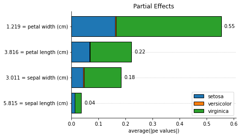
Explaining the IT_classifier expression using Partial Effects
Now let’s create an instance of ITExpr_explainer.
We can calculate feature importances with Partial Effects (PE) or approximate the Shapley values using PE. There is also support to use Integrated Gradients as a feature importance method.
[9]:
# First lets create and fit the explainer with training data

explainer = ITExpr_explainer(
    itexpr=final_itexpr,
    tfuncs=tfuncs
).fit(X_train, y_train)
[10]:
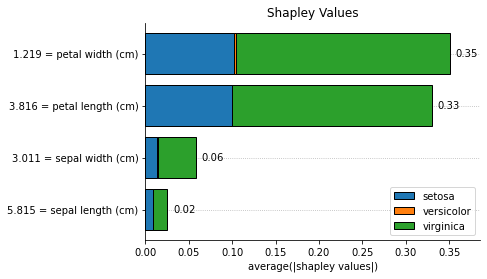
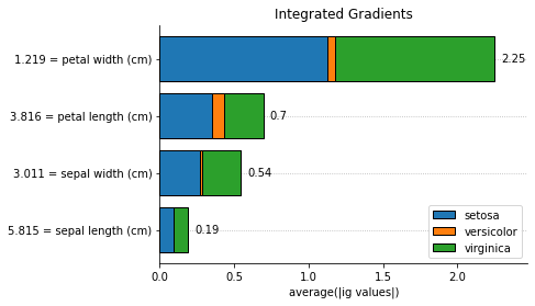
for method, method_name in [
    ('pe',      'Partial Effects'),
    ('shapley', 'Shapley Values'),
    ('ig',      'Integrated Gradients')
]:
    explainer.plot_feature_importances(
        X = X_train,
        importance_method = method,
        grouping_threshold = 0.0,
        target = None,
        barh_kw = {'edgecolor' : 'k'},
        show = False
    )

    # when we call a plot function, the explainers' axes_
    # will be the axes of the last plot. we called the plot function
    # with show=False to access the plot to add a title and then
    # we explicitly used the show() method to display the plots
    explainer.axes_.set_title(method_name)
    plt.show()
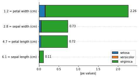
We can explain a single instance as well:
[11]:
explainer.plot_feature_importances(
    X = X_test[0, :].reshape(1, -1),
    importance_method = 'pe', # change to 'shapley'
    grouping_threshold = 0.0,
    target = None,
    barh_kw = {'edgecolor' : 'k'},
    show = True
)
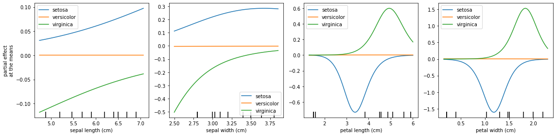
Instead of looking into the average Partial Effects, we can plot the Partial Effects for each variable when its co-variables are fixed at the means.
One phenomenon that can occur in a multiclassification problem is to have one class being a baseline, which is observed below. This explains why the feature importance shoud be summed for all classes.
[12]:
fig, axs = plt.subplots(1, 4, figsize=(16, 4))

explainer.plot_partial_effects_at_means(
    X          = X_test, # Obtaining explanations for test data
    ax         = axs,
    features   = final_itexpr.labels,
    target     = None,
    num_points = 100,
    share_y    = False,
    show_err   = False,
    show       = False,
)

plt.tight_layout()
plt.show()
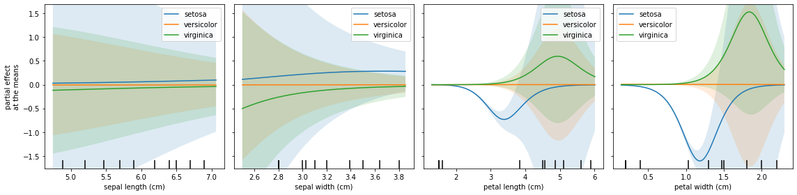
We can share the y axis and show errors hatchs:
[13]:
fig, axs = plt.subplots(1, 4, figsize=(16, 4))

explainer.plot_partial_effects_at_means(
    X          = X_test, # Obtaining explanations for test data
    ax         = axs,
    features   = final_itexpr.labels,
    target     = None,
    num_points = 100,
    share_y    = True,
    show_err   = True,
    show       = False,
)

plt.tight_layout()
plt.show()
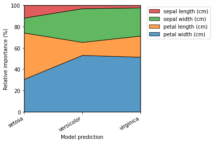
[14]:
explainer.plot_normalized_partial_effects(grouping_threshold=0.1, show=False)

plt.tight_layout()
plt.show()
In this example, wew didn’t specified the dictionary with the derivatives of every t ransformation function. ITExpr_explainer will use jax library to automatically infer the derivatives, as long as you have used jax.numpy instead of the traditional numpy.
This means that, after fitting the ITExpr_explainer, we have an dictionary of the vectorized version of the derivatives for each transformation function!
[15]:
# printing the derivative of sin, without having to implement it by hand
# (remember that is a vectorized function, and the input should be a np array)
print(
    explainer.tfuncs_dx['log'](
        np.array([1.0, 2.0, 3.0])
    )
)
[1. 0.5 0.33333334]